LAMMPS SPH演化与重启续算

本篇接着SPH压力与相向黏性，把同一四粒子模型从零步力计算推进到0.001s，查看密度变化，再演示实际重启续算。它是理解输入、状态和续算的最小例，不是实际水流动或收敛输运性质模型。

1. 一次运行共同例子#

下载完整SPH输入、脚本与结果图包，解压进入 lammps-sph-dynamics，在已分配CPU作业内执行：

bash run.sh

也可 sbatch job.slurm 提交。CPU分区按56核整节点分配和计费，本例一个线程；使用 lammps/30Sep2026-8173m 的普通CPU路径，oneAPI2024.2构建，绘图用 sisl/0.16.4。CPU队列维护时待恢复再提交，不在登录节点运行生产模拟。

流程为：连续100步 → 前半50步写restart → 从restart再跑50步 → 同一进程两个50步的对照 → 比较和绘图。四次原生调用合计300积分步，属于同一个SPH模型，不是四种独立方法。

2. 从完整输入理解密度演化#

cat inputs/continuous.lmp

units si
atom_style sph
boundary f f f
region box block 0 0.1 0 0.1 0 0.1 units box
create_box 1 box
create_atoms 1 single 0.03 0.04 0.05 units box
create_atoms 1 single 0.05 0.04 0.05 units box
create_atoms 1 single 0.04 0.06 0.05 units box
create_atoms 1 single 0.04 0.05 0.07 units box
mass 1 0.01
set group all sph/rho 1100
set group all sph/e 0
set group all sph/cv 1
comm_modify vel yes
neighbor 0.002 bin
neigh_modify delay 0 every 1 check yes
velocity all set 0 0 0 units box
pair_style sph/taitwater
pair_coeff * * 1000 10 1 0.03
variable vx atom "-0.2*(x-0.05)"
variable vy atom "-0.2*(y-0.05)"
variable vz atom "-0.2*(z-0.05)"
velocity all set v_vx v_vy v_vz units box
compute rho all sph/rho/atom
compute u all sph/e/atom
fix int all sph
timestep 0.00001
thermo 1
thermo_style custom step atoms
thermo_modify format float %.17g
dump tr all custom 1 trajectory.dump id type x y z vx vy vz fx fy fz c_rho c_u
dump_modify tr sort id format float %.17g
run 100
write_restart final.restart

初始每个粒子质量0.01kg、密度1100kg/m³、比热参数1，采用Tait状态方程、声速参数10m/s、参考密度1000kg/m³和核长度0.03m。fix sph 同时推进位置、速度、密度和内部能。初始弱相向速度并不意味着整个过程中始终压缩，压力力也会改变运动。

100步后四个粒子的密度约为 1072.504、1072.504、1075.186、1084.613kg/m³。这里的四点不是一个有完整边界和充分邻居的真实水体，因此这些密度只用于追踪例子中的状态变化。

3. 保存与读取重启文件#

前半段运行50步后执行 write_restart final.restart。后半段完整输入如下：

cat inputs/second-half.lmp

read_restart ../first-half/final.restart
pair_style sph/taitwater
pair_coeff * * 1000 10 1 0.03
comm_modify vel yes
neighbor 0.002 bin
neigh_modify delay 0 every 1 check yes
compute rho all sph/rho/atom
compute u all sph/e/atom
fix int all sph
timestep 0.00001
thermo 1
thermo_style custom step atoms
thermo_modify format float %.17g
dump tr all custom 1 trajectory.dump id type x y z vx vy vz fx fy fz c_rho c_u
dump_modify tr sort id format float %.17g
run 50
write_restart final.restart

sph/taitwater 不会把势参数写入restart。 读取restart后必须重新指定原来的 pair_style 和 pair_coeff。计算、输出与积分器也要按续算需要设置，不是只写一句 read_restart 就可以跑完。邻居通信仍保留 comm_modify vel yes。

4. 怎样正确比较续算轨迹#

cat results/SUMMARY.json
head -n 6 results/evolution.csv

当前版本的 fix sph 在每次 run 初始化时把预测速度 vest 设为当前速度 v。因此，不中断一次跑100步与50步后重启再跑50步存在微小差别。这个例子后50步的最大坐标差约2.73×10⁻⁹m，最大密度差约2.06×10⁻⁴kg/m³；不能宣称两者逐帧完全相同。

使用同样的run边界做对照，即同一进程先 run 50 再 run 50，其第51至100步与restart续算的全部输出一致。这说明比较精确续算时，需要同时匹配算法初始化方式。

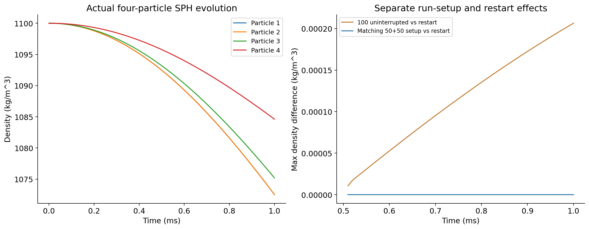
第50步“前段结束时的力”和“后段初始化后的力”属于两个数值阶段，即使位置、速度和密度已恢复，速度相关力仍可不同。合并输出时要保留这一边界含义，不能把同编号记录无说明地混成一帧。

5. 重画与换自己的模型#

module load sisl/0.16.4
python -B verify.py --reference
python -B plot.py

这些命令只处理已有结果，不重新积分。results/evolution.csv 给出每步时间、密度范围、动能和内部能等；本例没有据短轨迹声称时间步、能量漂移或材料输运精度已收敛。换自己的模型时，还要检查粒子间距/核长度、邻居数、状态方程、时间步、边界条件和所需的连续性精度。